When moving through cities we pass many different places and areas. Parks, shopping malls, residential areas. Ever wondered how this relates to your daily commute? I was. So with help of geopandas and Osmnx I tried to firgue this out.

Now the place where I do most of my moving around is Amsterdam. With my bike as my vehicle of choice.

Luckily for me, OSMnx (a python module made by Geoff Boeing) lets you download street network data. Although this is not always fully updated, for this exercise right here it does the trick.
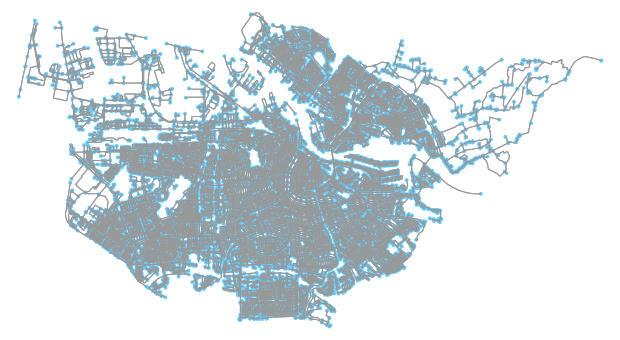
G = ox.graph_from_place('Amsterdam, Netherlands',network_type='walk')

Since I want to work with addresses instead of coordinates I’ll use the Amsterdam openAPI to translate these addresses into coordinates. Subsequently, these coordinates will help me find the nodes in OSMnx closest to the chosen addresses.

def send_request_loc(adres):
# GET https://api.data.amsterdam.nl/bag/openbareruimte/
    response = requests.get(
        url="https://api.data.amsterdam.nl/atlas/search/adres/",
        params={"q": adres,},)
    resp_str = response.content
    resp_dict = json.loads(resp_str)
    if len(resp_dict['results']) == 0:
        coord = ['Geen gegevens']
    else:
        coord = resp_dict['results'][0]['centroid']
    
    return coord

Using the openAPI we can get the coordinates of the start en end point of our route. In this case I’m using the route from Amsterdam Central train station to one of my frequent work places, the Amsterdam East municipal district office.

loc1 = send_request_loc('Stationsplein')
loc2 = send_request_loc('Linnaeuskade 31')node1 = ox.distance.nearest_nodes(G,loc1[0],loc1[1])
node2 = ox.distance.nearest_nodes(G,loc2[0],loc2[1])

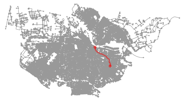
Using both locations, we can plot the shortest path with OSMnx.

route = nx.shortest_path(G, node1, node2,weight='length')
ox.plot_graph_route(G, route)

To get a bit of the surroundings for our route, we should create a buffer around it. To do so I first collected a LineString representing the route:

line = []
for i in route:
    point = (G.nodes[i]['x'],G.nodes[i]['y'])
    line.append(point)line = LineString(line)

Next step is to make this LineString into a GeoDataFrame in order to draw a buffer around it.

#creating a dataframe with the route information
route_df = pd.DataFrame(data= [['route 1',line]],columns=['naam_route','geometry'])#transforming dataframe to a geodataframe
route_df = gpd.GeoDataFrame(route_df,geometry='geometry')#creating a buffer around the route
route_df.geometry = route_df.geometry.buffer(0.0002)

Now the goal was not only to plot the route. But also get an idea of what kind of surfaces we are passing while commuting these routes. To do so, we’ll use the ‘Land Use’ map. Available on the the Amsterdam data portal (https://data.amsterdam.nl/datasets/It8vygqzGAantA/grondgebruik/).

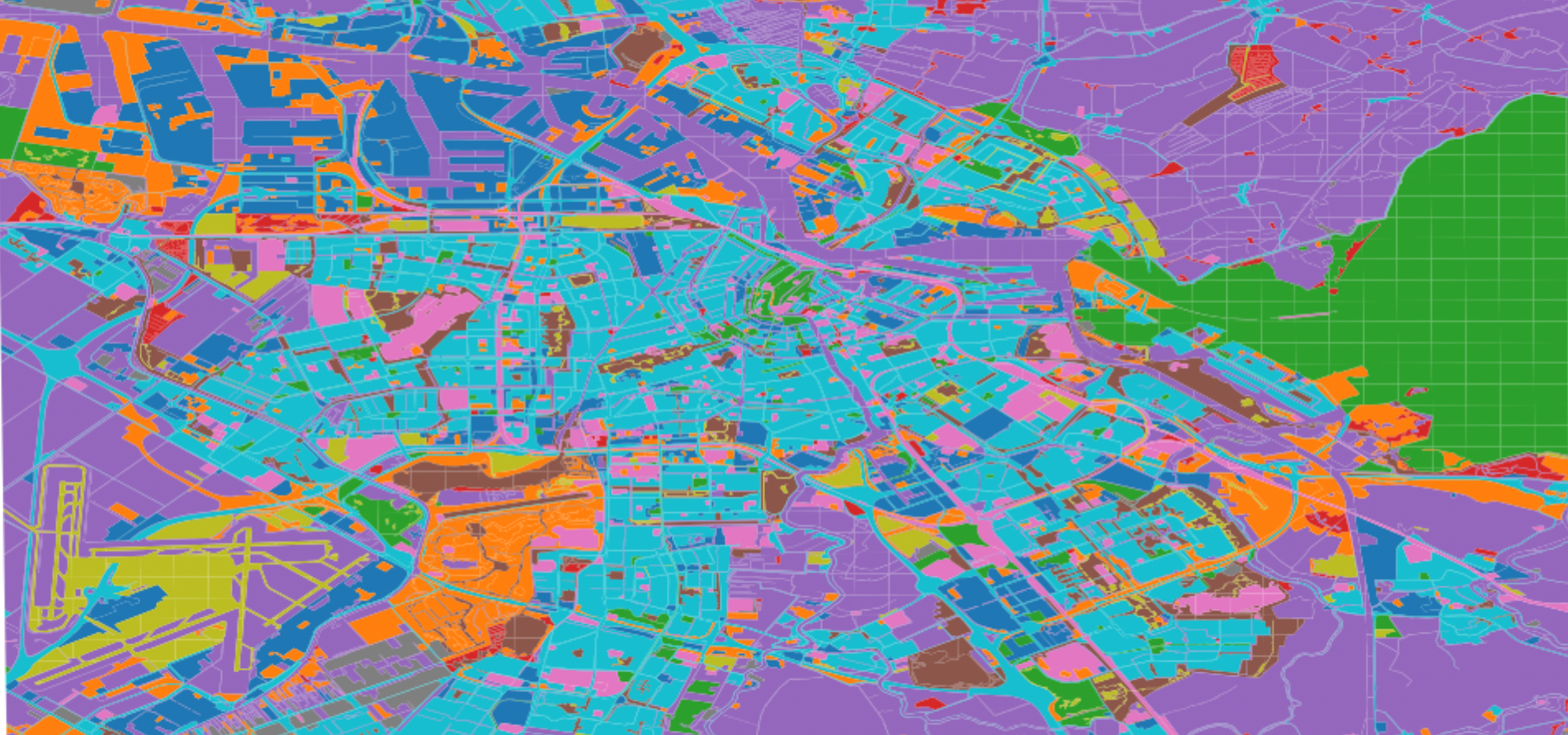
The map above shows the land use in different parts of the city. With each color showing a different kind of land use, including examples like forest, metro lines and recreational waters. By using a spacial join w can now see what kind of terrains the buffer of our route passes.

joined_gdf = gpd.sjoin(gdf, route_df, op='intersects')

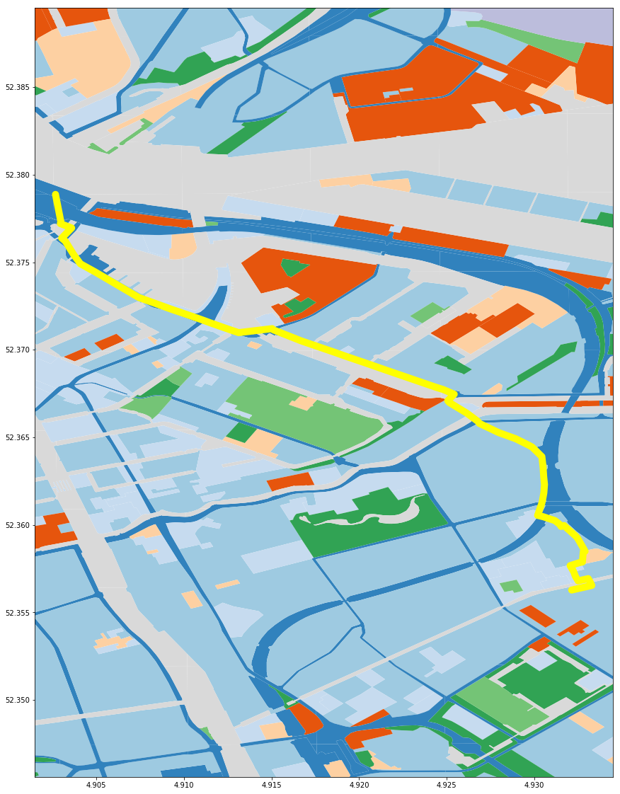
Visualized it will look like this:

After setting creating the route, setting the buffer and joining the geodataframes, it is time to see how what kind of land use intersects with the buffer of our route. To do so we loop over every unique patch of land use we cross, and calculate how much area we are intersecting. Finally we sum all these intersections per land use, and calculate it as a percentage by deviding it by the total area we cross and multiplying it with 100.

area = []
for i in joined_gdf.geometry:
    ar = i.intersection(route_df.iloc[0].geometry).area
    area.append(ar)joined_gdf['area'] = areaintersection = pd.DataFrame(joined_gdf.groupby(['AMScode_Oms'])['area'].sum())area_sum = intersection.area.sum(axis=0)intersection['percentage_land_use'] = intersection['area'] / area_sum * 100

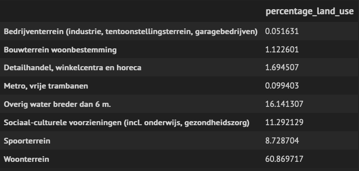
Finally we drop all ‘Wegverkeersterrein’ (road traffic area) since this is not part of the scenery. Leaving us with the following table:

Not really a green route. So next step would be to optimize the route based on our preferences. Whether this is patches of green, old monuments, or quite streets.

More information on OSMnx here. Check out the Amsterdam openAPI’s here. (in Dutch though). And see my Github for the full code. Note: The libraries and data used in this example is neither the most up-to-date, nor the best way to tackle the given problem. However it is a nice and simple way to do so.